Welcome to the LTER interactive cartographic almanac.
This document provides simple instructions on how to use the almanac and brief descriptions of the data layers for the National Map (48 contiguous states) and the World Map (North America with insets for Moorea and Antarctica LTER sites).
- National Atlas (.pdf, 65 MB)
- World Atlas (.pdf, 165 MB)
These PDF files contain layers that can be turned off and on (displayed or hidden) and can be saved or exported in other formats and inserted into a document or presentation. After the file is downloaded it can be opened in Adobe Acrobat, Adobe Illustrator or Adobe Photoshop. These instructions are specific to Adobe Acrobat. The file initially opens with several default layers displayed. To see a list of all the available layers in the PDF, click on the Layers Icon. The small box on the left side of each layer title will display an eye symbol if the layer is visible and will be empty if the layer is hidden. Click on the empty boxes to make the hidden layers visible. The layers are ordered hierarchically (ie. layers higher on the list will be displayed above lower layers). Some layers have legends associated with them, so only one of these layers can be displayed at a time.
World Atlas Layers
Layers are listed in the order they appear in the world atlas followed by brief description and citation if needed.
LTER Sites Labels: This map layer has point locations of all LTER sites with three letter site acronyms outlined in white.
LTER Domains: This map layer has study regions of all LTER sites outlined in red.
Continents outline: This map layer contains the outlines of continents only.
North America Countries:This map layer has outlines of the Continents and the outlines of the Countries of North America combined.
North American States: This map layer has outlines of the area near Moorea, Antarctica, and the outlines of the all the states and provinces of North America combined.
Major Rivers:This map layer contains the major rivers a North America
Watersheds of North America: This map was created by the FAO-UN by delineating drainage basin boundaries from hydrologically corrected elevation data (HydroSHEDS and Hydro1K). Input data resolution is 15 arc-seconds between 60 N and 60 S latitude (based on SRTM), and 30 arc-seconds for higher latitudes (based on GTOPO30). For complete metadata see http: //www.fao.org/geonetwork/srv/en/metadata.show?id=38047
2000 Population Density: The Global Rural-Urban Mapping Project, Version 1 (GRUMPv1) consists of estimates of human population for the year 2000 by 30 arc-second (1km) grid. The population density grids measure population per square km. A proportional allocation gridding algorithm, utilizing more than 1,000,000 national and sub-national geographic units, is used to assign population values to grid cells. The population count grids are divided by the land area grid to produce population densities. This dataset is produced by the Columbia University Center for International Earth Science Information Network (CIESIN) in collaboration with the International Food Policy Research Institute (IFPRI), The World Bank, and Centro Internacional de Agricultura Tropical (CIAT). Citation: Socioeconomic Data and Applications Center (SEDAC), Columbia University (2011). For complete metadata see: http: //sedac.ciesin.columbia.edu/downloads/metadata/grump-v1-population-density.html
2015 Population Density: Gridded Population of the World, Version 3 (GPWv3) Future Estimates consists of estimates of human population for the year 2015 by 2.5 arc-minute grid cells and associated datasets dated circa 2000. A proportional allocation gridding algorithm, utilizing more than 300,000 national and sub-national administrative units, is used to assign population values to grid cells. The population counts that the grids are derived from are extrapolated based on a combination of subnational growth rates from census dates and national growth rates from United Nations statistics. All of the grids have been adjusted to match United Nations national level population estimates. The population count grids contain estimates of the number of persons per grid cell. Citation: Socioeconomic Data and Applications Center (SEDAC), Columbia University (2005). For complete metadata see: http: //sedac.ciesin.columbia.edu/downloads/metadata/gpw-v3-population-density-future-estimates.html
AVHRR 8KM Classification: The University of Maryland Department of Geography generated this global land cover classification collection in 1998. Imagery from the AVHRR satellites acquired between 1981 and 1994 were analyzed to distinguish fourteen land cover classes. Citation: Hansen, M., R. DeFries, J.R.G. Townshend, and R. Sohlberg (1998), UMD Global Land Cover Classification, 8 Kilometer, 1.0, Department of Geography, University of Maryland, College Park, Maryland, 1981-1994. For complete metadata see: http: //www.glcf.umd.edu/data/landcover/description.shtml.
AVHRR 1KM Classification: The University of Maryland Department of Geography generated this global land cover classification collection in 1998. Imagery from the AVHRR satellites acquired between 1981 and 1994 were analyzed to distinguish fourteen land cover classes. Citation: Hansen, M., R. DeFries, J.R.G. Townshend, and R. Sohlberg (1998), UMD Global Land Cover Classification, 1 Kilometer, 1.0, Department of Geography, University of Maryland, College Park, Maryland, 1981-1994. For complete metadata see: http: //www.glcf.umd.edu/data/landcover/description.shtml
Modis Classification: The MODIS Land Cover Type product (2003) is derived from observations spanning a year’s input of Terra and Aqua data. The land cover scheme identifies 17 land cover classes defined by the International Geosphere Biosphere Programme (IGBP), which includes 11 natural vegetation classes, 3 developed and mosiacked land classes, and three non-vegetated land classes. For complete metadata see: http: //mercury.ornl.gov/ornldaac/send/xsltText2?fileURL=d%3A%5Cmercury_instances%5Cornldaac%5Crgd%5Charvested%5Crecord263.xml&full_datasource=Regional+and+Global+Data&full_queryString=+%28+title+%3A+MODIS+%28MCD12Q1%29+Land+Cover+Product+%29+AND+%28+datasource+%3A%28+rgd++%29+%29+&ds_id=Created+20101104+052449+by+66.82.162.21
Ecoregions Bailey-Division: Bailey Ecoregions Map of the Continents characterizes global climate and potential natural vegetation at approximately 1/2-degree resolution. The data set is based on a Russian vegetation map (Gerasimov, 1964) which was updated by the U.S. Fish and Wildlife Service (Robert G. Bailey), however the geographic projection was unknown. This version was reprojected to geodetic coordinates at the World Conservation Monitoring Center, England. The data set consists of one independent spatial layer with three attributes. Citation: Bailey, R.G. and H.C. Hogg, 1986. A world ecoregions map for resource reporting. Environmental Conservation, Vol. 13, No. 3, pp. 195-202. Bailey, R.G. 1989. Explanatory supplement to Ecoregions Map of the Continents. Environmental Conservation, vol. 16, no. 4, pp 307-309. For complete metadata see: http: //www.ngdc.noaa.gov/ecosys/cdroms/ged_iib/datasets/b03/bec.htm
Ecoregions Bailey-Domain: Bailey Ecoregions Map of the Continents characterizes global climate and potential natural vegetation at approximately 1/2-degree resolution. The data set is based on a Russian vegetation map (Gerasimov, 1964) which was updated by the U.S. Fish and Wildlife Service (Robert G. Bailey), however the geographic projection was unknown. This version was reprojected to geodetic coordinates at the World Conservation Monitoring Center, England. The data set consists of one independent spatial layer with three attributes. Citation: Bailey, R.G. and H.C. Hogg, 1986. A world ecoregions map for resource reporting. Environmental Conservation, Vol. 13, No. 3, pp. 195-202. Bailey, R.G. 1989. Explanatory supplement to Ecoregions Map of the Continents. Environmental Conservation, vol. 16, no. 4, pp 307-309. For complete metadata see: http: //www.ngdc.noaa.gov/ecosys/cdroms/ged_iib/datasets/b03/bec.htm
Global Landcover: The Global Vegetation Monitoring Unit carries out several activities related to Land Cover mapping and monitoring. In particular the GVM Unit is coordinating and implementing the Global Land Cover 2000 Project (GLC 2000) in collaboration with a network of partners around the world. The general objective is to provide for the year 2000 a harmonized land cover database over the whole globe. To achieve this objective GLC 2000 makes use of the VEGA 2000 dataset: a dataset of 14 months of pre-processed daily global data acquired by the VEGETATION instrument on board the SPOT 4 satellite, made available through a sponsorship from members of the VEGETATION programme, including JRC. Citation: Global Land Cover 2000 database. European Commission, Joint Research Centre, 2003, http: //www-gem.jrc.it/glc2000. For complete metadata see: http: //bioval.jrc.ec.europa.eu/products/glc2000/products/GLC2000_EUR_20849EN.pdf
Eco Zones: The 2000 global ecological zone map has been developed, building upon the FRA 1990 experience for the tropics and extending the coverage to include the temperate and boreal forests. A globally consistent classification has been adopted, based on the Koppen-Trewartha climate system in combination with natural vegetation characteristics. A total of 19 global ecological zones have been defined and mapped, ranging from the evergreen tropical rainforest zone to the boreal tundra woodland zone. A main principle of delineating the global ecological zones involved the aggregation or matching of available regional ecological or potential vegetation maps into the global framework. Along with the core information on state and changes in forests, FRA 2000 is reporting on various ecological aspects of forests. Forest resources information will be reported by ecological zone, which will contribute to understanding the implications of forest change on (ecosystem) biological diversity and carbon-cycling processes. For complete metadata see: http: //www.fao.org/geonetwork/srv/en/metadata.show?id=1255
Olson’s Ecosystems: In 1980, this data base and the corresponding map were completed after more than 20 years of field investigations, consultations, and analyses of published literature. They characterize the use and vegetative cover of the Earth’s land surface with a 0.5° × 0.5° grid. This world-ecosystem-complex data set and the accompanying map provide a current reference base for interpreting the role of vegetation in the global cycling of CO2 and other gases and a basis for improved estimates of vegetation and soil carbon, of natural exchanges of CO2, and of net historic shifts of carbon between the biosphere and the atmosphere. Citation Olson, J.S., J.A. Watts, and L.J. Allison. 1985. Major world ecosystem complexes ranked by carbon in live vegetation: A Database. NDP-017, Carbon Dioxide Information Center, Oak Ridge National Laboratory, Oak Ridge, Tennessee. doi: 10.3334/CDIAC/lue.ndp017 (Revised 2001). For complete metadata see: http: //cdiac.ornl.gov/epubs/ndp/ndp017/ndp017.html#abstract
Biomes: This map depicts terrestrial ecoregions of the globe. Ecoregions are relatively large units of land containing distinct assemblages of natural communities and species, with boundaries that approximate the original extent of natural communities prior to major land-use change. This comprehensive, global map provides a useful framework for conducting biogeographical or macroecological research, for identifying areas of outstanding biodiversity and conservation priority, for assessing the representation and gaps in conservation efforts worldwide, and for communicating the global distribution of natural communities on earth. Biomes have increasingly been adopted by research scientists, conservation organizations, and donors as a framework for analyzing biodiversity patterns, assessing conservation priorities, and directing effort and support (Ricketts et al. 1999a; Wikramanayake et al. 2001; Ricketts et al. 1999b; Olson & Dinerstein 1998; Groves et al. 2000; Rosenzweig et al. 2003; and Luck et al. 2003). More on the approach to ecoregion mapping, the logic and design of the framework, and previous and potential uses are discusses in Olson et al. (2001) and Ricketts et al. (1999a). Citation: Olson, D.M., E. Dinerstein, E.D. Wikramanayake, N.D. Burgess, G.V.N. Powell, E.C. Underwood, J.A. D’Amico, I. Itoua, H.E. Strand, J.C. Morrison, C.J. Loucks, T.F. Allnutt, T.H. Ricketts, Y. Kura, J.F. Lamoreux, W.W. Wettengel, P. Hedao, and K.R. Kassem. Terrestrial Ecoregions of the World: A New Map of Life on Earth (PDF, 1.1M) BioScience 51: 933-938.
Number of Endemic: The number of terrestrial endemic species refers to the number of endemic mammals, birds, and reptiles in each terrestrial ecoregion. Data was compiled on endemic species by querying the WWF WildFinder database for their occurrences by ecoregion. The WWF WildFinder database is a spatially explicit online database of vertebrate species occurrences by ecoregion. Citation: Terrestrial Endemic Species Richness by ecoregion: World Wildlife Fund (WWF). 2006. WildFinder: Database of species distributions, ver. Jan-06. Available at www.gis.wwf.org/WildFinder
Number of Mammals: Data was compiled on terrestrial mammals by querying the WWF WildFinder database for species occurrences by ecoregion. The WWF WildFinder database is a spatially explicit online database of vertebrate species occurrences by ecoregion. Citation: Mammal Species Richness by ecoregion: World Wildlife Fund (WWF). 2006. WildFinder: Database of species distributions, ver. Jan-06. Available at www.gis.wwf.org/WildFinder
Number of Birds: Data was compiled on terrestrial birds by querying the WWF WildFinder database for species occurrences by ecoregion. The WWF WildFinder database is a spatially explicit online database of vertebrate species occurrences by ecoregion. Citation: Bird Species Richness by ecoregion: World Wildlife Fund (WWF). 2006. WildFinder: Database of species distributions, ver. Jan-06. Available at www.gis.wwf.org/WildFinder.
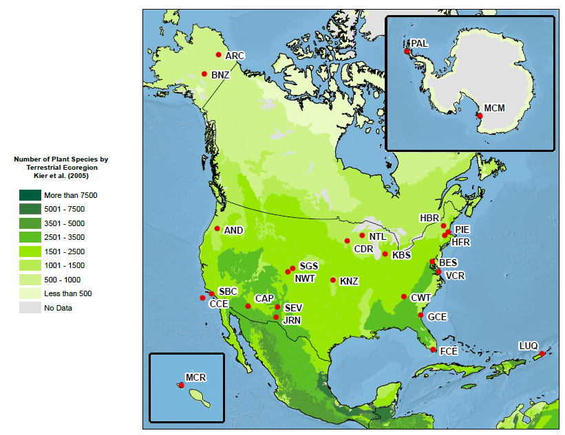
Number of Plants: Kier et al. (2005) estimated the number of plant species in each terrestrial ecoregion. Citation: Plant Species Richness by ecoregion: Kier, G., J. Mutke, E. Dinerstein, T. H. Ricketts, W. Ku, H. Kreft, and W. Barthlott. 2005. Global patterns of plant diversity and floristic knowledge. Journal of Biogeography 32: 1107-1116.
Plant hardiness zones: The Plant Hardiness images were generated by Jay Schlegel of ZedX Inc, using two sources of weather data for the NCSU APHIS Plant Pest Forecast System. One source is the International Program on Climate Change (IPCC) 1973-2002 monthly data consisting of maximum and minimum temperatures and precipitation (New et al., 1999). The second source is the Daily Global Historical Climatology Network (GHCND) station data that contains daily values of maximum and minimum temperature and precipitation for more than 33,000 locations worldwide (Peterson and Vose, 1997). Citation: NAPPFAST Global Plant Hardiness Zones. July, 2007. North Carolina State University APHIS Plant Pest Forecasting System, <http: //www.nappfast.org>.
Soils of the World: Soil information, from the global to the local scale, has often been the one missing biophysical information layer, the absence of which has added to the uncertainties of predicting potentials and constraints for food and fiber production. The lack of reliable and harmonized soil data has considerably hampered land degradation assessments, environmental impact studies and adapted sustainable land management interventions. Recognizing the urgent need for improved soil information worldwide, particularly in the context of the Climate Change Convention and the Kyoto Protocol for soil carbon measurements and the immediate requirement for the FAO/IIASA Global Agro-ecological Assessment study (GAEZ 2008), the Food and Agriculture Organization of the United Nations (FAO) and the International Institute for Applied Systems Analysis (IIASA) took the initiative of combining the recently collected vast volumes of regional and national updates of soil information with the information already contained within the 1: 5,000,000 scale FAO-UNESCO Digital Soil Map of the World, into a new comprehensive Harmonized World Soil Database (HWSD). The completion of this comprehensive harmonized soil information will improve estimation of current and future land potential productivity, help identify land and water limitations, and enhance assessing risks of land degradation, particularly soil erosion. The HWSD contributes sound scientific knowledge for planning sustainable expansion of agricultural production and for guiding policies to address emerging land competition issues concerning food production, bio-energy demand and threats to biodiversity. This is of critical importance for rational natural resource management and in making progress towards achieving Millennium Development goals of eradicating hunger and poverty and addressing the food security and sustainable agricultural development, especially with regard to the threats of global climate change and the needs for adaptation and mitigation. This soil information system will allow policy makers, planners and experts to overcome some of the shortfalls of data availability to address the old challenges of food production and food security and plan for new challenges of climate change and accelerated natural resources degradation. Citation: FAO/IIASA/ISRIC/ISS-CAS/JRC, 2009. Harmonized World Soil Database (version 1.1). FAO, Rome, Italy and IIASA, Laxenburg, Austria.
Permafrost Distribution: Permafrost distribution for Arctic regions was derived from the original 1: 10,000,000 paper map (Brown et al. 1997). Permafrost distribution for Antarctica was derived from (Bockheim, J.G. and K.J. Hall. 2002).
Land Surface Temp: Land surface temperature is how hot the “surface” of the Earth would feel to the touch in a particular location. From a satellite’s point of view, the “surface” is whatever it sees when it looks through the atmosphere to the ground. It could be snow and ice, the grass on a lawn, the roof of a building, or the leaves in the canopy of a forest. Thus, land surface temperature is not the same as the air temperature that is included in the daily weather report. The map was made using data collected during the daytime by the Moderate Resolution Imaging Spectroradiometer (MODIS) on NASA’s Terra satellite. At mid-to-high latitudes, land surface temperatures can vary throughout the year, but equatorial regions tend to remain consistently warm, and Antarctica and Greenland remain consistently cold. Altitude plays a clear role in temperatures, with mountain ranges like the North American Rockies cooler than other areas at the same latitude. Scientists monitor land surface temperature because the warmth rising off Earth’s landscapes influences (and is influenced by) our world’s weather and climate patterns. Scientists want to monitor how increasing atmospheric greenhouse gases affect land surface temperature, and how rising land surface temperatures affect glaciers, ice sheets, permafrost, and the vegetation in Earth’s ecosystems. Commercial farmers may also use land surface temperature maps like these to evaluate water requirements for their crops during the summer, when they are prone to heat stress. Conversely, in winter, these maps can help citrus farmers to determine where and when orange groves could have been exposed to damaging frost.
NDVI July 2011: Satellites observe global-scale patterns of vegetation that scientists use to study changes in plant growth as a result of climate and environmental changes as well as human activity. Photosynthesis plays a big role in removing carbon dioxide from the atmosphere and storing it in wood and soils, so mapping vegetation is a key part of studying the carbon cycle. Farmers and resource managers also use satellite-based vegetation maps to help them monitor the health of our forests and croplands. On this map, vegetation is pictured as a scale, or index,of greenness. Greenness is based on several factors: the number and type of plants, how leafy they are, and how healthy they are. In places where foliage is dense and plants are growing quickly, the index is high, represented in dark green. Regions where few plants grow have a low vegetation index, shown in tan. The index is based on measurements taken by the Moderate Resolution Imaging Spectroradiometer (MODIS) on NASA’s Terra satellite.
Ocean Temp AVHRR: Sea surface temperature is the temperature of the top millimeter of the ocean’s surface, which scientists call the "skin temperature." Like Earth’s land surface, sea surface temperatures are warmer near the equator and colder near the poles. Currents like giant rivers move warm and cold water around the world’s oceans. Some of these currents flow on the surface, and they are obvious in sea surface temperature images. Ocean temperatures influence weather, including hurricanes, the productivity of marine plant and animal life, and the rate at which carbon dioxide in the air dissolves in the waters of the ocean. Over long periods of time, changes in sea surface temperature are indicators of natural and human-caused climate change. Changes in ocean surface temperatures have a huge impact on weather and land. For example, when the full width of the Pacific heats up along the equator, an El Niño develops. El Niño alters rainfall patterns around the globe, causing heavy rainfall in the southern United States and severe drought in Australia, Indonesia, and southern Asia. On a smaller scale, ocean temperatures influence the development of tropical cyclones (hurricanes and typhoons), which need warm ocean waters to form and grow. Ocean temperatures also influence how quickly tiny ocean plants can grow. Since the plants absorb carbon dioxide as they turn sunlight into energy, they influence how much carbon dioxide the oceans can soak up. Scientists who want to measure how much carbon dioxide is in the atmosphere and how much is absorbed by plants are interested in the connection between sea surface temperatures and ocean plant growth. These data have been collected since 1981 by a series of National Oceanic and Atmospheric Administration (NOAA) satellites.
Ocean Temp MODIS: Sea surface temperatures have a large influence on climate and weather. For example, every 3 to 7 years a wide swath of the Pacific Ocean along the equator warms by 2 to 3 degrees C. This warming is a hallmark of the climate pattern El Niño, which changes rainfall patterns around the globe, causing heavy rainfall in the southern United States and severe drought in Australia, Indonesia, and southern Asia. On a smaller scale, ocean temperatures influence the development of tropical cyclones (hurricanes and typhoons), which draw energy from warm ocean waters to form and intensify. These sea surface temperature maps are based on observations by the Moderate Resolution Imaging Spectroradiometer(MODIS) on NASA’s Aqua satellite.
Snow and Ice: This map shows the maximum extent of snow and sea ice for both the Arctic and Antarctic winters.
Oceans only: This Ocean Basemap includes bathymetry, surface and subsurface feature names, and derived depths. This map is designed to be used as a basemap layer,
Physical earth: This layer is combination of shaded relief and land cover; intended for use as a basemap layer.
ESRI Shaded Relief: Surface elevation presented as shaded relief; intended for use as a basemap layer.
ESRI World Imagery: This layer presents satellite imagery for the world.
Earth at Night: This image of Earth’s city lights that was created with data from the Defense Meteorological Satellite Program (DMSP) Operational Linescan System (OLS). Originally designed to view clouds by moonlight, the OLS is also used to map the locations of permanent lights on the Earth’s surface. Data was acquired October 1, 1994 – March 31, 1995. Citation: NASA’s Earth Observatory
National Map Layers
Layers are listed in the order they appear in the atlas followed by brief description and citation if needed.
LTER Sites: This map layer has point locations of LTER sites with three letter site acronyms that are located within the boundary of the 48 contiguous states.
LTER Sites w/ Mask: This map layer has point locations of LTER sites with three letter site acronyms outlined in white that are located within the boundary of the 48 contiguous states.
Other Research Sites: This map layer is a combination of three data sets: location of core NEON sites, NADP sites, and Biological Field Stations.
State and Province Boundaries: This map layer show outlines of Mexican States, Canadian Providences, and the 48 contiguous states.
US States Only: This map layer contains shows outlines of the 48 contiguous states only.
Regional Watersheds Outline: This map layer contains hydrologic unit boundaries and codes for the United States. It was revised for inclusion in the National Atlas of the United States of America, and updated to match the streams file created by the USGS National Mapping Division (NMD) for the National Atlas of the United States of America. This is a revised version of the November 2002 map layer. Citation: National Atlas of the United States.
Subregional Watersheds Outline: This map layer contains hydrologic unit boundaries and codes for the United States. It was revised for inclusion in the National Atlas of the United States of America, and updated to match the streams file created by the USGS National Mapping Division (NMD) for the National Atlas of the United States of America. This is a revised version of the November 2002 map layer. Citation: National Atlas of the United States.
US Rivers Major: This map layer shows major rivers of the United States.
US Rivers Minor: This map layer shows areal and linear water features of the United States. The original file was produced by joining the individual State hydrography layers from the 1: 2,000,000- scale Digital Line Graph (DLG) data produced by the USGS. This map layer was formerly distributed as Hydrography Features of the United States. This is a revised version of the January 2003 map layer. Citation: National Atlas of the United States.
Bailey’s Ecoregions by Division: This map layer is commonly called Bailey’s ecoregions and shows ecosystems of regional extent in the United States. Four levels of detail are included to show a hierarchy of ecosystems. The largest ecosystems are domains, which are groups of related climates and which are differentiated based on precipitation and temperature. Divisions represent the climates within domains and are differentiated based on precipitation levels and patterns as well as temperature. Also identified are mountainous areas that exhibit different ecological zones based on elevation. Citation: National Atlas of the United States.
Bailey’s Ecoregions by Providence: This map layer is commonly called Bailey’s ecoregions and shows ecosystems of regional extent in the United States. Four levels of detail are included to show a hierarchy of ecosystems. The largest ecosystems are domains, which are groups of related climates and which are differentiated based on precipitation and temperature. Divisions represent the climates within domains and are differentiated based on precipitation levels and patterns as well as temperature. Divisions are subdivided into provinces, which are differentiated based on vegetation or other natural land covers. Also identified are mountainous areas that exhibit different ecological zones based on elevation. Citation: National Atlas of the United States.
Omernik ecoregions Level 3: This map layer shows Omernik’s Level III ecoregions, derived from a 1: 7,500,000 map created by J.M. Omernik in 1987 and from refinements of Omernik’s framework that were made for other projects. Ecoregions describe areas of general similarity in ecosystems and in the type, quality, and quantity of environmental resources. Omernik’s ecoregions are based on the premise that a hierarchy of ecological regions can be identified through the analysis of the patterns and the composition of both living and nonliving phenomena, such as geology, physiography, vegetation, climate, soils, land use, wildlife, and hydrology, that affect or reflect differences in ecosystem quality and integrity. All the characteristics are considered when determining ecoregions, but the relative importance of each characteristic may vary from one ecoregion to another. Level III is the most detailed level available nationally for this system of ecoregions. Citation: National Atlas of the United States.
Geology: This data set contains boundaries for major geologic units in the United States. The data depict the geology of the bedrock that lies at or near the land surface, but not the distribution of surficial materials such as soils, alluvium, and glacial deposits. This is a revised version of the April 2004 data set. The data are generalized from a compilation prepared for use in the Geologic Map of North America, to be published in hard copy by the Geological Society of America and released as a digital file by the U.S. Geological Survey. Citation: National Atlas of the United States.
Regional Watersheds w/ Legend: This map layer contains hydrologic unit boundaries and codes for the United States. It was revised for inclusion in the National Atlas of the United States of America, and updated to match the streams file created by the USGS National Mapping Division (NMD) for the National Atlas of the United States of America. This is a revised version of the November 2002 map layer. Citation: National Atlas of the United States.
Subregional Watersheds Filled: This map layer contains hydrologic unit boundaries and codes for the United States. It was revised for inclusion in the National Atlas of the United States of America, and updated to match the streams file created by the USGS National Mapping Division (NMD) for the National Atlas of the United States of America. This is a revised version of the November 2002 map layer. Citation: National Atlas of the United States.
NEON Domains: NEON Domain’s located within the boundary of the 48 contiguous states.
PRISM Avg Min Temp 1971-2000: This map layer contains spatially gridded average annual minimum temperature for the climatological period 1971-2000. Distribution of the point measurements to a spatial grid was accomplished using the PRISM model, developed and applied by Chris Daly of the PRISM Climate Group at Oregon State University. Citation: PRISM Climate Group, Oregon State University, http: //prism.oregonstate.edu.
PRISM Avg Max Temp 1971-2000: This map layer contains spatially gridded average annual maximum temperature for the climatological period 1971-2000. Distribution of the point measurements to a spatial grid was accomplished using the PRISM model, developed and applied by Chris Daly of the PRISM Climate Group at Oregon State University. Citation: PRISM Climate Group, Oregon State University, http: //prism.oregonstate.edu.
PRISM Avg Annual Precip 1971-2000: This map layer contains spatially gridded average monthly and annual precipitation for the climatological period 1971-2000. Distribution of the point measurements to a spatial grid was accomplished using the PRISM model, developed and applied by Chris Daly of the PRISM Climate Group at Oregon State University. Citation: PRISM Climate Group, Oregon State University, http: //prism.oregonstate.edu.
Federal land ownership: This map layer consists of federally owned or administered lands of the United States and Indian Lands of the United States. Only areas of 640 acres or more are included. There may be private inholdings within the boundaries of Federal lands in this map layer. Federally-administered lands within a reservation are included for continuity; these may or may not be considered part of the reservation and are simply described with their feature type and the administrating Federal agency. This is a revised version of the December 2005 map layer. Citation: National Atlas of the United States
Forest types: This map layer portrays general forest cover types for the United States. Data were derived from Advanced Very High Resolution Radiometer (AVHRR) composite images recorded during the 1991 growing season. A total of 25 classes of forest cover types were interpreted from the AVHRR, aided by field observations and refined with ancillary data from digital elevation models. Citation: National Atlas of the United States.
Land Cover Classes: This map layer is land cover characteristics for United States. The nominal spatial resolution is 1 km and the map layer is based on Advanced Very High Resolution Radiometer (AVHRR) data. The data were compiled by staff at the National Center for Earth Resources Observation and Science as part of the Global Land Cover Characterization Project. The land cover classes were produced using data from April 1992 to March 1993. Documentation and the original data are available at <http: //edcsns17.cr.usgs.gov/glcc/>. Citation: National Atlas of the United States.
NADP Total N Deposition: 2010 Inorganic nitrogen wet deposition from nitrate and ammonium from qualifying National Atmospheric Deposition Program, National Trends Network sites. Citation: National Atmospheric Deposition Program 2011. NADP Program Office, Illinois State Water Survey, 2204 Griffith Dr., Champaign, IL 61820.
Map Box Outline: This layer is a simple black outline around the map.
Shaded relief: Surface elevation presented as shaded relief; intended for use as a basemap layer.
Physical earth: This layer is combination of shaded relief and land cover; intended for use as a basemap layer.
Background: North America colored tan with all water blue and 48 contiguous states outlined; intended for use as a basemap layer.